2 Data preprocessing
2.1 Data import: GPS and raster data
I start by importing GPS data of adults only (without individuals from the Jacksonville zoo), in the form of trajectories (ltraj) that is converted to point data (SpatialPointsDataFrame) and projected to Lat/Long:
library("hab")
load("Data/wost-ad-ltraj.RData")
library("rgdal")
wost <- hab::ltraj2spdf(trajad, strict = FALSE, proj4string = CRS("+init=epsg:32617"))
wost$id <- factor(wost$id)
wost <- subset(wost, !(id %in% c(407680, 429200, 476550, 721310, 721320)))
wost <- spTransform(wost, CRS("+proj=longlat +datum=WGS84"))
summary(wost)
## Object of class SpatialPointsDataFrame
## Coordinates:
## min max
## x -91.45783 -78.01650
## y 25.08267 34.60033
## Is projected: FALSE
## proj4string :
## [+proj=longlat +datum=WGS84 +ellps=WGS84 +towgs84=0,0,0]
## Number of points: 445638
## Data attributes:
## date dx dy
## Min. :2005-07-29 07:00:00 Min. :-90334.77 Min. :-127323.69
## 1st Qu.:2007-09-28 19:00:00 1st Qu.: -30.13 1st Qu.: -19.90
## Median :2009-07-09 17:00:00 Median : 0.00 Median : 0.00
## Mean :2009-04-11 15:12:47 Mean : 5.56 Mean : -12.55
## 3rd Qu.:2010-10-29 20:00:00 3rd Qu.: 31.28 3rd Qu.: 19.58
## Max. :2011-12-31 18:00:00 Max. :133219.05 Max. : 148420.54
## NA's :36011 NA's :36011
## dist dt R2n
## Min. : 0.00 Min. :3600 Min. : 0
## 1st Qu.: 16.76 1st Qu.:3600 1st Qu.: 108970
## Median : 49.76 Median :3600 Median : 9802756
## Mean : 1544.56 Mean :4777 Mean : 24050154883
## 3rd Qu.: 639.01 3rd Qu.:7200 3rd Qu.: 1192219334
## Max. :150312.14 Max. :7200 Max. :1005475966130
## NA's :36011 NA's :22863
## abs.angle rel.angle id burst
## Min. :-3.14 Min. :-3.14 572931 : 29866 414590 : 21736
## 1st Qu.:-1.57 1st Qu.:-1.57 414590 : 21736 414240 : 18336
## Median : 0.00 Median : 0.15 414240 : 18336 414580 : 14595
## Mean : 0.09 Mean : 0.18 721290 : 16319 416110 : 14110
## 3rd Qu.: 1.57 3rd Qu.: 2.04 723560 : 15763 407700 : 13064
## Max. : 3.14 Max. : 3.14 414580 : 14595 414260 : 12473
## NA's :110418 NA's :143287 (Other):329023 (Other):351324
## gid elevation day
## Min. :148996 Min. :-999.0 Min. : 429
## 1st Qu.:293034 1st Qu.: 3.0 1st Qu.:1220
## Median :456866 Median : 10.0 Median :1870
## Mean :442556 Mean :-173.2 Mean :1781
## 3rd Qu.:584878 3rd Qu.: 28.0 3rd Qu.:2347
## Max. :701216 Max. :2032.0 Max. :2775
## NA's :22873wost2 <- droplevels(wost@data)
length(unique(wost2$id))## [1] 61table(wost2$id)##
## 407700 407710 414240 414250 414260 414270 414580 414590 414600 414610
## 13064 1463 18336 5676 12473 2523 14595 21736 8671 628
## 416100 416110 425120 429190 475171 475180 475192 475220 475241 475270
## 651 14110 5093 11316 2683 11720 650 2137 19 4867
## 475282 475284 475302 475322 519770 519790 519800 519810 572661 572662
## 1790 1245 2729 505 8973 7306 8909 7876 3998 3839
## 572671 572710 572741 572742 572743 572781 572800 572811 572931 572951
## 1083 10281 346 2268 3202 4386 1098 5881 29866 7911
## 572981 572991 721290 721300 723560 723570 723580 723600 723610 809320
## 4614 8626 16319 9859 15763 2824 2134 2910 7459 5638
## 809330 809340 910200 910210 910220 910230 910240 992250 992270 992280
## 805 9165 13990 14474 14269 14105 3372 9188 7607 8761
## 992290
## 7853summary(as.numeric(table(wost2$id)))## Min. 1st Qu. Median Mean 3rd Qu. Max.
## 19 2523 5881 7306 10280 29870sd(as.numeric(table(wost2$id)))## [1] 6036.537summary(unlist(by(wost2, wost2$id, function(k) difftime(max(k$date), min(k$date),
units = "days"))))## Min. 1st Qu. Median Mean 3rd Qu. Max.
## 1.25 247.50 527.50 649.10 972.30 2326.00sd(unlist(by(wost2, wost2$id, function(k) difftime(max(k$date), min(k$date),
units = "days"))))## [1] 562.5885I also import environmental data (from files). All rasters are combined in a RasterBrick, which is then masked using a Minimum convex polygon (from adehabitatHR) of every relocations enlarged by a one-cell buffer:
library("raster")
janPrec <- raster("Data/Consensus_rasters/jan_prec.img")
janTemp <- raster("Data/Consensus_rasters/jan_temp.img")
febPrec <- raster("Data/Consensus_rasters/feb_prec.img")
febTemp <- raster("Data/Consensus_rasters/feb_temp.img")
marPrec <- raster("Data/Consensus_rasters/mar_prec.img")
marTemp <- raster("Data/Consensus_rasters/mar_temp.img")
aprPrec <- raster("Data/Consensus_rasters/apr_prec.img")
aprTemp <- raster("Data/Consensus_rasters/apr_temp.img")
mayPrec <- raster("Data/Consensus_rasters/may_prec.img")
mayTemp <- raster("Data/Consensus_rasters/may_temp.img")
junPrec <- raster("Data/Consensus_rasters/jun_prec.img")
junTemp <- raster("Data/Consensus_rasters/jun_temp.img")
julPrec <- raster("Data/Consensus_rasters/jul_prec.img")
julTemp <- raster("Data/Consensus_rasters/jul_temp.img")
augPrec <- raster("Data/Consensus_rasters/aug_prec.img")
augTemp <- raster("Data/Consensus_rasters/aug_temp.img")
sepPrec <- raster("Data/Consensus_rasters/sep_prec.img")
sepTemp <- raster("Data/Consensus_rasters/sep_temp.img")
octPrec <- raster("Data/Consensus_rasters/oct_prec.img")
octTemp <- raster("Data/Consensus_rasters/oct_temp.img")
decPrec <- raster("Data/Consensus_rasters/dec_prec.img")
decTemp <- raster("Data/Consensus_rasters/dec_temp.img")
novPrec <- raster("Data/Consensus_rasters/nov_prec.img")
novTemp <- raster("Data/Consensus_rasters/nov_temp.img")
(rast <- brick(janPrec, janTemp, febPrec, febTemp, marPrec, marTemp, aprPrec,
    aprTemp, mayPrec, mayTemp, junPrec, junTemp, julPrec, julTemp, augPrec,
    augTemp, sepPrec, sepTemp, octPrec, octTemp, novPrec, novTemp, decPrec,
    decTemp))
## class : RasterBrick
## dimensions : 855, 2156, 1843380, 24 (nrow, ncol, ncell, nlayers)
## resolution : 0.167, 0.167 (x, y)
## extent : -180, 180.052, -59.1665, 83.6185 (xmin, xmax, ymin, ymax)
## crs : NA
## source : /tmp/Rtmp4OILip/raster/r_tmp_2019-10-30_173244_13787_41238.grd
## names : jan_prec, jan_temp, feb_prec, feb_temp, mar_prec, mar_temp, apr_prec, apr_temp, may_prec, may_temp, jun_prec, jun_temp, jul_prec, jul_temp, aug_prec, ...
## min values : 0.00, -51.45, 0.00, -47.45, 0.00, -44.55, 0.00, -35.75, 0.00, -19.80, 0.00, -13.55, 0.00, -10.85, 0.00, ...
## max values : 808.90, 33.10, 714.15, 32.45, 689.05, 32.25, 632.15, 33.90, 965.00, 35.80, 2136.30, 38.35, 2123.25, 38.20, 1538.70, ...library("rgeos")
sa <- mcp(wost, percent = 100)
rast <- crop(rast, gBuffer(sa, width = 0.167))
rast <- mask(rast, gBuffer(sa, width = 0.167))The result is something like this (using temperatures in January as an example)
library("sf")
library("maps")
states <- st_as_sf(map("state", plot = FALSE, fill = TRUE))
rastDF <- data.frame(rasterToPoints(rast))
library("cowplot")
library("viridis")
ggplot() + geom_raster(data = rastDF, aes_string(x = "x", y = "y", fill = names(rastDF)[4])) +
    geom_sf(data = states, fill = NA, size = 0.2, colour = gray(0.2)) + geom_point(data = data.frame(wost),
    aes(x = x, y = y), shape = 20, size = 0.8, stroke = 0, colour = "gray") +
    coord_sf(xlim = c(-92, -77.5), ylim = c(24.5, 35), expand = FALSE) + scale_fill_viridis(end = 0.8,
    alpha = 1, option = "plasma") + labs(x = "Latitude", y = "Longitude", fill = expression(`Temperature `(degree ~
    C))) + theme(legend.position = "top", legend.justification = "center") +
    guides(fill = guide_colourbar(barwidth = 15, barheight = 1, title.theme = element_text(size = 26)))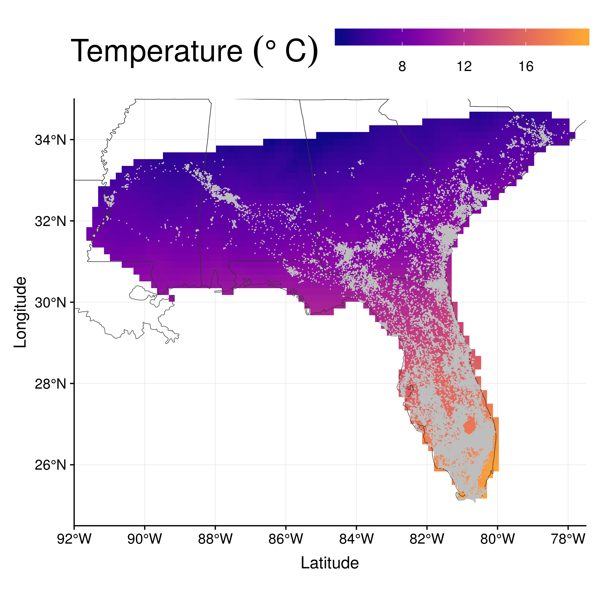
Figure 2.1: Temperature in January.
2.2 Environmental intersection
We first look at the frequency of data for each month:
library("lubridate")
wost$month <- month(wost$date)
table(wost$month)
##
## 1 2 3 4 5 6 7 8 9 10 11 12
## 28931 26156 30298 33741 40787 38467 42136 44483 43625 42663 38409 35942plot(table(wost$month), ylab = "Frequency", xlab = "Month")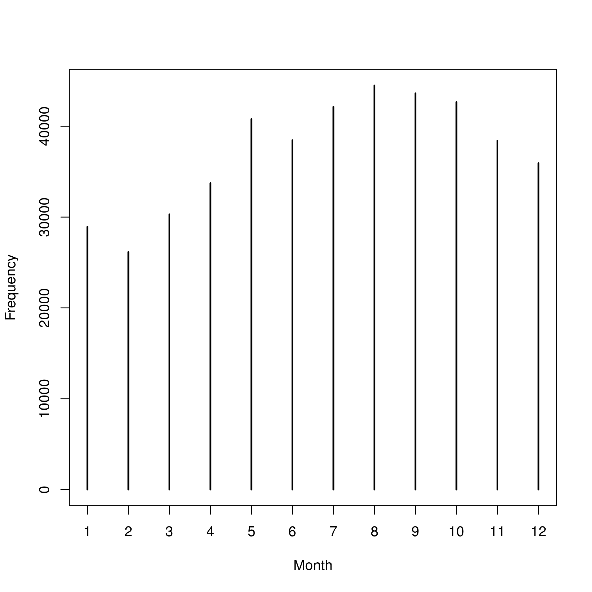
Figure 2.2: Frequency of data per month.
We then intersect the GPS data to the precipitation and temperature layers, using the month number to identify the correct layer:
wost$prec <- ifelse(wost$month == 1, extract(janPrec, wost),
    ifelse(wost$month == 2, extract(febPrec, wost),
        ifelse(wost$month == 3, extract(marPrec, wost),
            ifelse(wost$month == 4, extract(aprPrec, wost),
                ifelse(wost$month == 5, extract(mayPrec, wost),
                    ifelse(wost$month == 6, extract(junPrec, wost),
                        ifelse(wost$month == 7, extract(julPrec, wost),
                            ifelse(wost$month == 8, extract(augPrec, wost),
                                ifelse(wost$month == 9, extract(sepPrec, wost),
                                    ifelse(wost$month == 10, extract(octPrec, wost),
                                        ifelse(wost$month == 11, extract(novPrec, wost),
                                            extract(decPrec, wost))))))))))))
wost$temp <- ifelse(wost$month == 1, extract(janTemp, wost),
    ifelse(wost$month == 2, extract(febTemp, wost),
        ifelse(wost$month == 3, extract(marTemp, wost),
            ifelse(wost$month == 4, extract(aprTemp, wost),
                ifelse(wost$month == 5, extract(mayTemp, wost),
                    ifelse(wost$month == 6, extract(junTemp, wost),
                        ifelse(wost$month == 7, extract(julTemp, wost),
                            ifelse(wost$month == 8, extract(augTemp, wost),
                                ifelse(wost$month == 9, extract(sepTemp, wost),
                                    ifelse(wost$month == 10, extract(octTemp, wost),
                                        ifelse(wost$month == 11, extract(novTemp, wost),
                                            extract(decTemp, wost))))))))))))
Note that the correlation between temperature and precipitation in wood stork use data is pretty high.
cor(wost$prec, wost$temp, use = "complete.obs")## [1] 0.7965986plot(wost$prec, wost$temp, pch = 20, xlab = "Precipitation", ylab = "Temperature")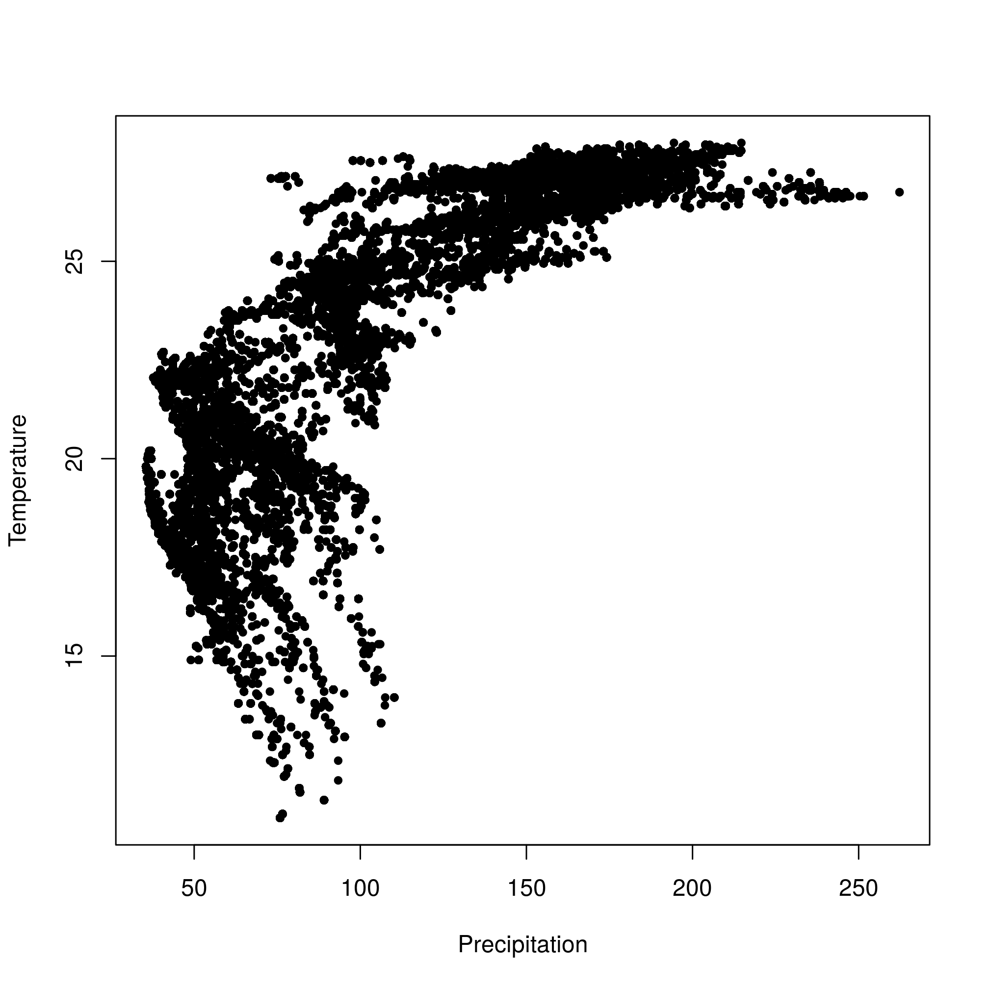
Figure 2.3: Correlation between precipitation and temperature.
2.3 Sampling the point data
In this section, I will sample GPS data to ensure that each individual is represented equally in each month. I first break down the data into a list with one element per month. Over this list, i.e. for each month, individuals with less than 100 locations are removed, and one random location of a random individual (with replacement) is chosen 5000 times, to give each individual the same weight in the sampled data:
table(wost$id, wost$month)##
## 1 2 3 4 5 6 7 8 9 10 11 12
## 407680 0 0 0 0 0 0 0 0 0 0 0 0
## 407700 956 856 897 911 1040 950 1325 1371 1211 1257 1295 995
## 407710 0 0 0 0 0 0 323 308 329 342 161 0
## 414240 1488 1328 1486 1490 1579 1595 1633 1638 1551 1555 1453 1540
## 414250 266 311 313 539 637 619 629 693 617 467 290 295
## 414260 947 739 781 1057 1232 1062 1207 1189 1087 1090 1040 1042
## 414270 0 0 0 175 317 320 337 327 308 348 319 72
## 414580 903 855 962 1390 1376 1416 1632 1504 1404 1233 945 975
## 414590 1530 1373 1637 1902 1980 1937 2058 1963 1927 1990 1840 1599
## 414600 620 556 554 872 887 809 801 872 778 728 615 579
## 414610 0 0 0 148 244 236 0 0 0 0 0 0
## 416100 0 0 36 285 330 0 0 0 0 0 0 0
## 416110 1005 883 1061 1269 1546 1250 1336 1348 1113 1163 1075 1061
## 425120 144 132 223 398 466 444 791 692 710 535 374 184
## 429190 890 718 851 847 952 887 1086 1122 1065 983 1013 902
## 429200 0 0 0 0 0 0 0 0 0 0 0 0
## 475171 41 10 279 302 424 491 285 302 174 175 114 86
## 475180 508 680 1148 1112 1206 1020 1210 1087 1090 982 968 709
## 475192 0 0 0 331 319 0 0 0 0 0 0 0
## 475220 94 68 172 242 229 221 217 232 194 208 195 65
## 475241 0 0 0 0 0 0 19 0 0 0 0 0
## 475270 277 238 623 659 670 652 530 476 262 142 217 121
## 475282 0 0 0 0 0 0 356 426 422 434 152 0
## 475284 0 0 0 20 155 150 156 155 150 154 150 155
## 475302 317 336 359 396 313 0 24 241 53 133 275 282
## 475322 0 0 0 0 0 0 0 58 437 10 0 0
## 476550 0 0 0 0 0 0 0 0 0 0 0 0
## 519770 457 411 487 452 703 887 926 945 912 952 895 946
## 519790 467 428 470 439 472 446 617 898 907 917 763 482
## 519800 462 412 475 432 655 907 959 947 914 936 877 933
## 519810 470 440 477 446 438 423 625 949 920 901 889 898
## 572661 213 0 0 365 469 319 465 468 456 455 336 452
## 572662 156 0 0 0 440 444 434 472 459 480 474 480
## 572671 0 0 0 385 454 244 0 0 0 0 0 0
## 572710 712 724 1151 1145 1186 1025 704 641 725 777 723 768
## 572741 0 0 0 0 0 0 0 131 215 0 0 0
## 572742 0 0 0 0 0 0 255 444 449 464 404 252
## 572743 429 384 45 0 427 201 117 214 371 422 250 342
## 572781 444 20 32 439 467 346 456 442 459 439 384 458
## 572800 0 0 115 136 121 194 201 245 86 0 0 0
## 572811 460 407 454 450 455 391 430 151 554 892 780 457
## 572931 2456 2360 2416 2385 2420 2141 2434 2611 2786 2727 2541 2589
## 572951 892 786 468 452 423 268 446 643 899 905 858 871
## 572981 464 396 466 403 408 208 42 481 453 433 442 418
## 572991 797 737 856 745 451 286 463 879 841 875 849 847
## 721290 959 1038 1366 1259 1352 1548 1745 1805 1782 1672 940 853
## 721300 804 864 909 826 684 664 909 900 847 815 781 856
## 721310 0 0 0 0 0 0 0 0 0 0 0 0
## 721320 0 0 0 0 0 0 0 0 0 0 0 0
## 723560 1101 1215 1345 1307 1405 1336 1351 1395 1358 1381 1301 1268
## 723570 0 0 0 120 360 323 355 351 354 368 321 272
## 723580 0 0 0 45 356 298 363 359 339 353 21 0
## 723600 0 0 0 120 361 326 370 363 356 369 360 285
## 723610 471 470 826 768 633 738 696 757 758 559 406 377
## 809320 439 410 461 457 647 465 473 476 452 456 454 448
## 809330 0 0 0 0 135 477 193 0 0 0 0 0
## 809340 891 588 453 434 576 830 909 926 852 900 901 905
## 910200 875 794 955 863 1340 1248 1342 1284 1296 1361 1334 1298
## 910210 913 844 924 887 1353 1309 1364 1377 1357 1406 1367 1373
## 910220 906 811 950 917 1371 1271 1367 1390 1331 1364 1338 1253
## 910230 930 819 935 906 1282 1252 1304 1319 1322 1364 1342 1330
## 910240 0 0 0 0 444 418 458 470 455 483 448 196
## 992250 445 434 460 472 813 923 948 964 942 954 900 933
## 992270 466 439 487 450 676 927 928 956 729 484 441 624
## 992280 431 407 457 441 657 911 922 918 904 916 890 907
## 992290 435 435 476 450 451 414 610 908 903 954 908 909summary(as.numeric(table(wost$id)))## Min. 1st Qu. Median Mean 3rd Qu. Max.
## 0 1876 5366 6752 9691 29870months <- split(wost, wost$month)
for (i in 1:length(months)) months[[i]]$id <- factor(months[[i]]$id)
monthLocs <- lapply(months, function(k) {
k <- nsubset(k, id, 100)
k$id <- factor(k$id)
lt <- split(k, k$id)
set.seed(34138)
sam <- sample(1:length(lt), 5000, replace = TRUE)
return(do.call("rbind", lapply(sam, function(x) {
lt[[x]][sample(1:nrow(lt[[x]]), 1), ]
})))
})
monthLocsAll <- do.call(rbind, monthLocs)
table(monthLocsAll$month)##
## 1 2 3 4 5 6 7 8 9 10 11 12
## 5000 5000 5000 5000 5000 5000 5000 5000 5000 5000 5000 5000Here is the result on the map of temperatures in January:
ggplot() + geom_raster(data = data.frame(rasterToPoints(rast)), aes_string(x = "x",
    y = "y", fill = names(rast)[4])) + geom_sf(data = states, fill = NA, size = 0.2,
    colour = gray(0.2)) + geom_point(data = data.frame(wost), aes(x = x, y = y),
    shape = 20, size = 0.8, stroke = 0, colour = "gray") + geom_point(data = subset(data.frame(monthLocsAll),
    month == 1), aes(x = x, y = y), shape = 15) + coord_sf(xlim = c(-92, -77.5),
    ylim = c(24.5, 35), expand = FALSE) + scale_fill_viridis(end = 0.8, alpha = 1,
    option = "plasma") + labs(x = "Latitude", y = "Longitude", fill = expression(`Temperature `(degree ~
    C))) + theme(legend.position = "top", legend.justification = "center") +
    guides(fill = guide_colourbar(barwidth = 15, barheight = 1, title.theme = element_text(size = 26)))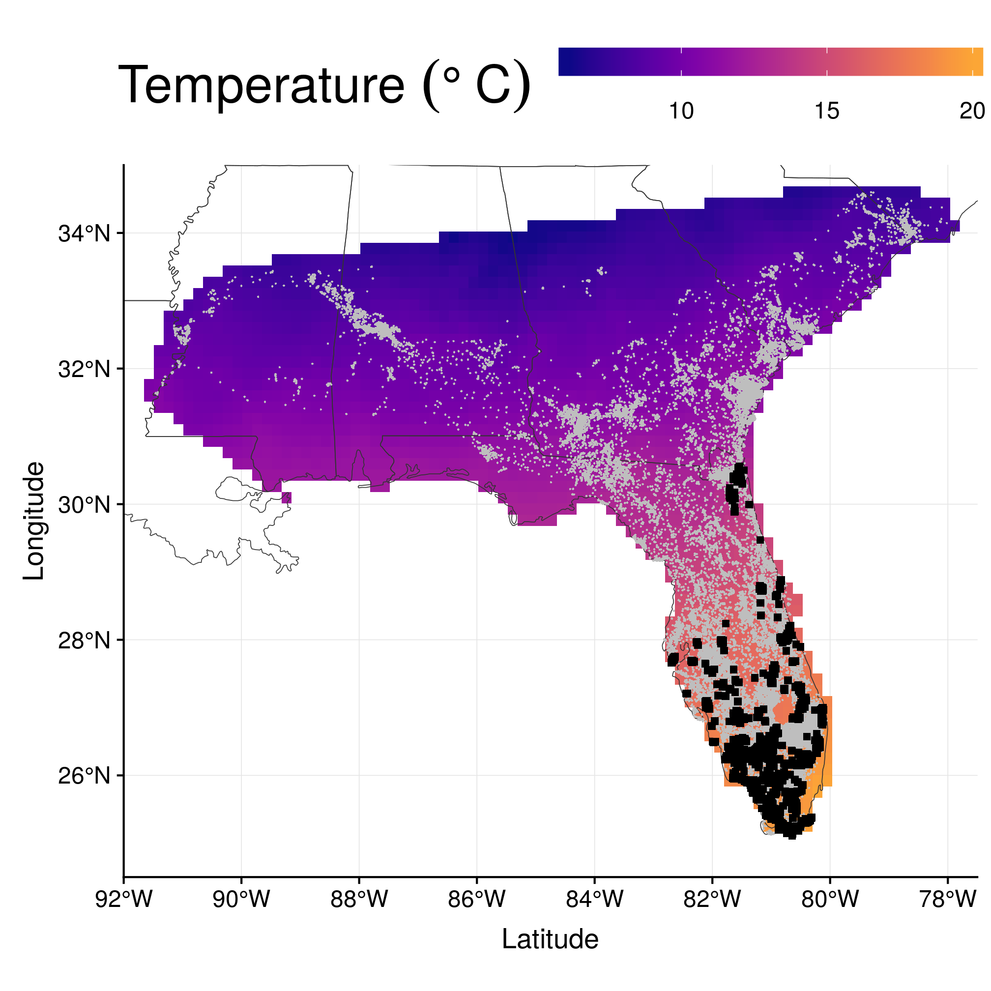
Figure 2.4: Wood stork location data (blue dots), with January temperatures in the background and January locations in black.